오늘의 목표
1. 1차 선형 회귀식 만들기
y = a * x1 + b * x2 + c
총점 = a * 수학 + b * 국어 + c
x1과 x2가 y를 결정하는 식이다.
즉, 수학점수와 국어점수가 총점을 결정한다고 이해하면 된다.
2. 수학, 국어 성적으로 총점을 예측하는 회귀식 만들기
x1 = 수학 성적
x2 = 국어 성적
y = 총점이다.
코드로 나타내보면 기본 선형 회귀와 같으나 x변수에서 math와 kor 두 가지를 모두 써주면 된다.
import pandas as pd
import openpyxl
import matplotlib.pyplot as plot
import sklearn
plot.rcParams["font.family"] = 'Malgun gothic'

data = pd.read_excel("student.xlsx", header=0)
print(data)
newData = data[['kor', 'eng', 'math', 'social', 'science', 'total']]

#속성(변수) 2가지 선택
x = newData[['math', 'kor']]
y = newData[['total']]

from sklearn.linear_model import LinearRegression

#단순 회귀 모델 생성
model = LinearRegression()
model.fit(x, y)

#예측 모델 생성
y_p = model.predict(x)

#가중치와 y절편 출력
print('가중치 a : ', model.coef_)
print('y절편 : ', model.intercept_)

#결정계수
relation_square = model.score(x, y)
print('결정계수 : ', relation_square)

#seaborn으로 나타내기
import seaborn as sns
ax1 = sns.distplot(y, hist = False, label = 'y실제')
ax2 = sns.distplot(y_p, hist = False, label = 'y예측')
plot.show()
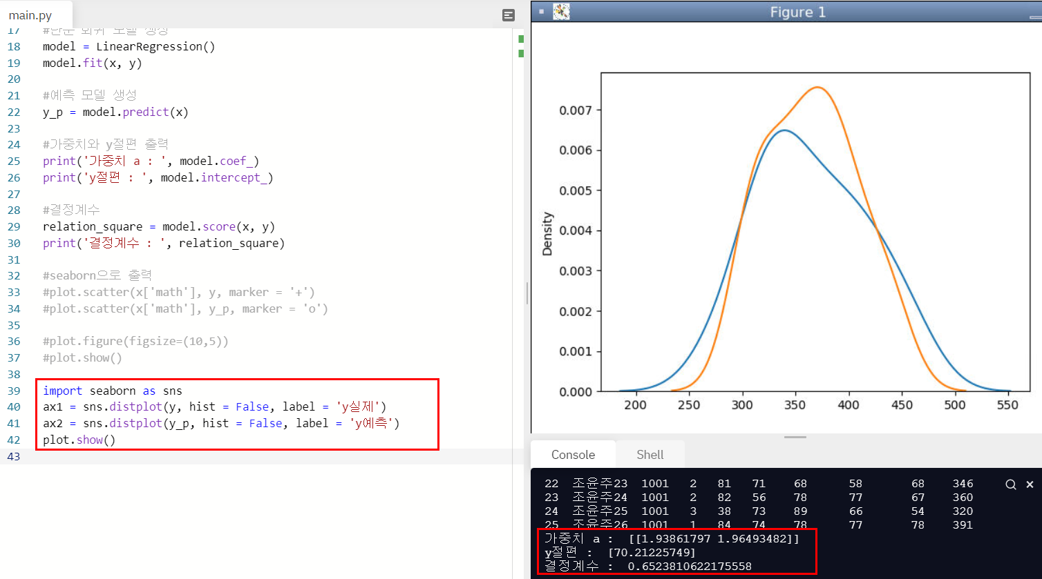
이렇게 되면
총점 = 1.93 * 수학 + 1.96 * 국어 + 70.212
라는 식이 탄생하고 결정계수는 0.652로 나오게 된다.
seaborn으로도 살펴보자.
3. 국어, 수학, 사회, 영어를 모두 넣어서 총점과의 관계를 살펴보는 선형 회귀식 만들기
이 경우에는 변수에 원하는 속성만 넣어주면 된다.
import pandas as pd
import openpyxl
import matplotlib.pyplot as plot
import sklearn
plot.rcParams["font.family"] = 'Malgun gothic'

data = pd.read_excel("student.xlsx", header=0)
print(data)
newData = data[['kor', 'eng', 'math', 'social', 'science', 'total']]

#속성(변수) 4가지 선택 : 수학, 국어, 영어, 사회
x = newData[['math', 'kor','eng', 'social']]
y = newData[['total']]

from sklearn.linear_model import LinearRegression

#단순 회귀 모델 생성
model = LinearRegression()
model.fit(x, y)

#예측 모델 생성
y_p = model.predict(x)

#가중치와 y절편 출력
print('가중치 a : ', model.coef_)
print('y절편 : ', model.intercept_)

#결정계수
relation_square = model.score(x, y)
print('결정계수 : ', relation_square)

#seaborn으로 출력
import seaborn as sns
ax1 = sns.distplot(y, hist = False, label = 'y실제')
ax2 = sns.distplot(y_p, hist = False, label = 'y예측')
plot.show()
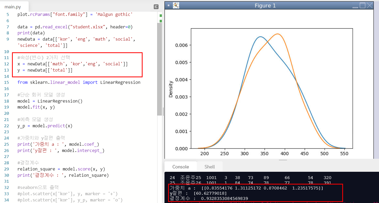
결과적으로 보면
0.83 * 수학 + 1.31 * 국어 + 0.87 * 영어 + 1.23 * 사회 = 총점
이라고 볼 수 있다.
결정계수는 0.932로 높게 나왔다.
국어, 사회, 영어, 수학 순서로 총점에 영향을 많이 미치는 것을 확인할 수 있다.
4. 2차 이상의 회귀식 만들기
수학, 국어 점수로 총점을 예상하는 2차 회귀식을 만들면
총점 = x * 수학 * 수학 + y * 수학 * 국어 + z * 국어 * 국어 + a * 수학 +b * 국어 + c
위의 식이 나온다.
import pandas as pd
import openpyxl
import matplotlib.pyplot as plot
import sklearn
plot.rcParams["font.family"] = 'Malgun gothic'

data = pd.read_excel("student.xlsx", header=0)
print(data)
newData = data[['kor', 'eng', 'math', 'social', 'science', 'total']]

#속성(변수) 2가지 선택
x = newData[['math', 'kor']]
y = newData[['total']]

from sklearn.linear_model import LinearRegression
from sklearn.preprocessing import PolynomialFeatures

poly = PolynomialFeatures(degree = 2) #2차항 적용
x_poly = poly.fit_transform(x)

#단순 회귀 모델 생성
model = LinearRegression()
model.fit(x_poly, y)

#예측 모델 생성
y_p = model.predict(x_poly)

#가중치와 y절편 출력
print('가중치 a : ', model.coef_)
print('y절편 : ', model.intercept_)

#결정계수
relation_square = model.score(x_poly, y)
print('결정계수 : ', relation_square)

import seaborn as sns
ax1 = sns.distplot(y, hist = False, label = 'y실제')
ax2 = sns.distplot(y_p, hist = False, label = 'y예측')
plot.show()
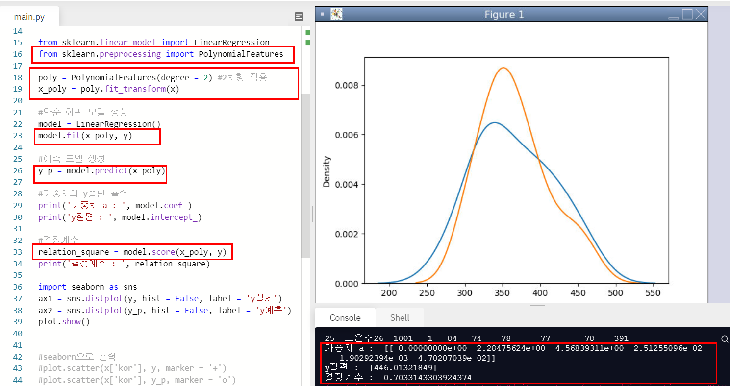
총점 = -2.28 * 수학 * 수학 -4.56 * 수학 * 국어 +2.51 * 국어 * 국어 +1.90 * 수학 + 4.70 * 국어 + 446.013
이라는 식이 도출되며
결정계수는 0.703이 나온다!
1차에서 결정계수는 0.652였는데 2차식으로 나타냈더니 0.703으로 높게 나왔다.
하지만 3차, 4차로 늘릴 수록 오히려 결정계수가 낮게 나오기도 하기에 적절한 n차식으로 나타내는 코드가 필요하다!
'프로그래밍 > 머신러닝' 카테고리의 다른 글
| 집값과 경기종합지수의 상관관계_파이썬으로 머신러닝 배우기 (0) | 2021.04.19 |
|---|---|
| 삼성전자, 현대자동차, LG화학 주가와 KOSPI 주가의 상관 관계 분석_파이썬으로 머신러닝 배우기 (0) | 2021.04.16 |
| 단순 선형 회귀 2차식, 3차식, n차식까지 만들기(PolynomialFeatures)_파이썬으로 머신러닝 배우기 (0) | 2021.04.12 |
| 단순 선형 회귀(LinearRegression)_파이썬으로 머신러닝 배우기 (1) | 2021.04.09 |
| Machine Learning이란? pip install 모듈 설치하기_파이썬으로 머신러닝 배우기 (0) | 2021.04.07 |


