앙상블(emsemble)
랜덤 포레스트(Random forest) 모델
1. 랜덤 포레스트(Random forest)란?
의사결정 트리를 랜덤하게 나온 것을 투표하여 결정하는 것이다.
분류, 회귀에 주로 사용된다.

Bagging Features
속성이 10개라고 10개 다 선정하는 것이 아니라
10을 제곱근 한 수 만큼 선정한다.
2. 분류 기준
엔트로피 이론
어떤 기준으로 가장 먼저 분류하면 좋을까?에 대해 고민할 때
보통 엔트로피 이론을 적용한다.

3. 랜덤 포레스트 인자 결정
n_estimator = 트리의 수
max_depth = 트리의 깊이
max_features = 나누는 수
n_estimator 는 클 수록 좋다! 트리를 많이 만들어 볼수록 좋다. (경우의 수가 많아진다.)
max_features 는 각 트리의 무작위를 얼마나 할 것인지 결정한다.
작은 max_features와 큰 n_estimator 는 과대 적합을 줄인다는 장점이 있다.
랜덤 포레스트 모델을 쓸 때는 n_estimator 인자와 max_features인자를 조절하며
결정계수가 가장 높아지는 인자를 사용하는 것이 좋다.
랜덤 포레스트 모델을 활용하면 분류와 회귀 모두 사용이 가능한데
분류를 할 때는 max_features = sqrt(n_features)
회귀 할 때는 max_features = n_features
를 써준다!
4. 랜덤 포레스트 모델 직접 사용해보기
x, y 데이터를 랜덤으로 만들어주고(지난 글과 같이 만들어준다.)
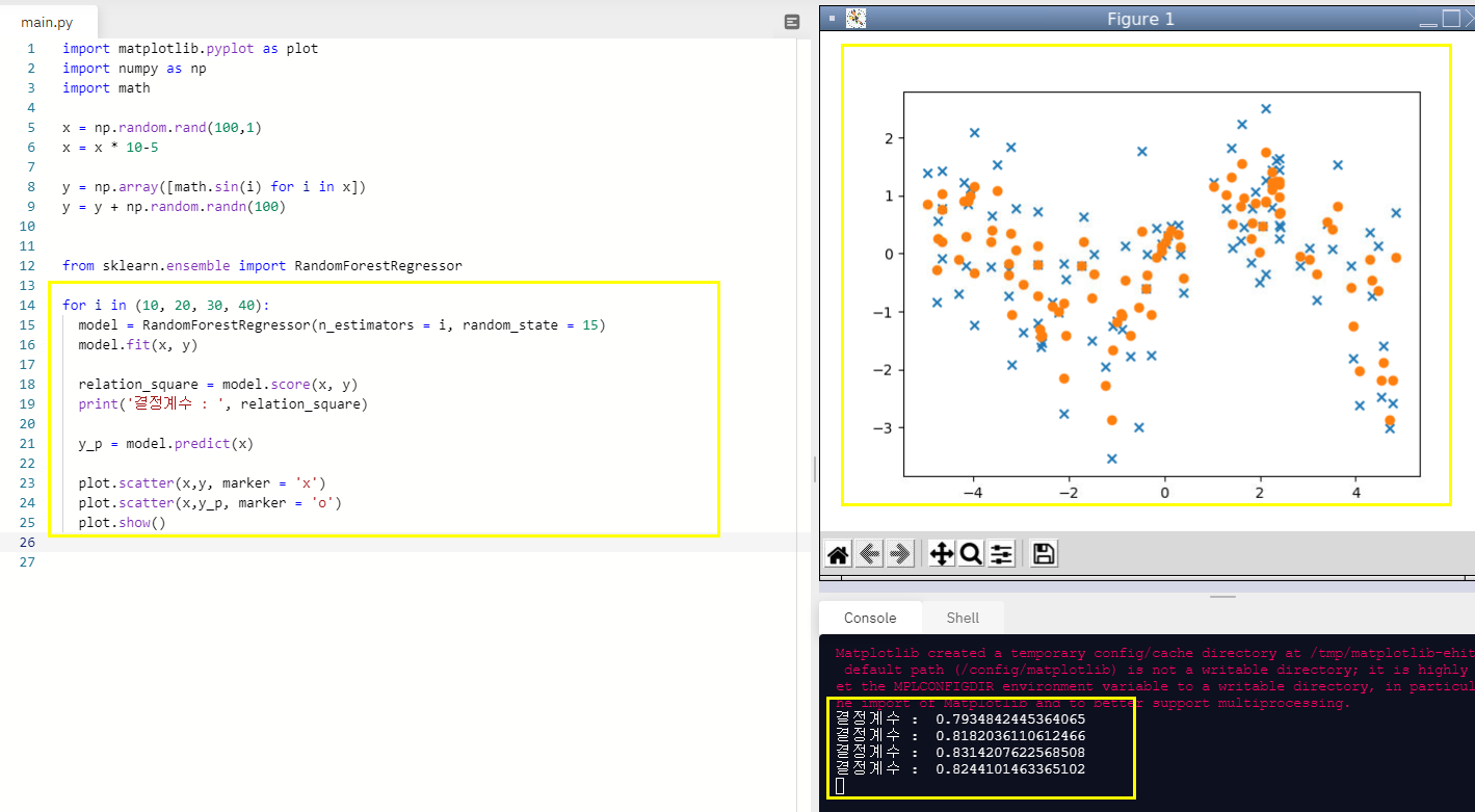
그 다음에 트리가 10, 20, 30, 40일때의 결정계수를 확인해보자.
import matplotlib.pyplot as plot
import numpy as np
import math

x = np.random.rand(100,1)
x = x * 10-5

y = np.array([math.sin(i) for i in x])
y = y + np.random.randn(100)

from sklearn.ensemble import RandomForestRegressor
#트리가 10개일때, 20일때, 30일때, 40일때
for i in (10, 20, 30, 40):
  model = RandomForestRegressor(n_estimators = i, random_state = 15)
  model.fit(x, y)

  relation_square = model.score(x, y)
  print('결정계수 : ', relation_square)

  y_p = model.predict(x)

  plot.scatter(x,y, marker = 'x')
  plot.scatter(x,y_p, marker = 'o')

  plot.show()
확인 결과 트리가 30일 때 즉, n_estimators가 30일 때 결정계수가 0.8244로 가장 높은 것을 볼 수 있다.
5. 이번에는 수학 점수로 총점을 예측해보자!
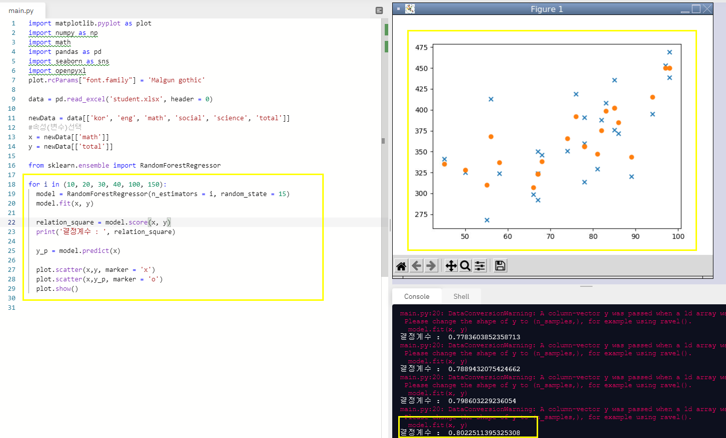
트리를 10, 20, 30, 40, 100, 150까지 반복해서 결정계수를 비교해보려한다.
student엑셀 파일도 지난 글에서 사용했던 파일을 그대로 썼고 수학 점수로 총점을 예측하고 그 때의 결정계수를 확인해보았다.
import matplotlib.pyplot as plot
import numpy as np
import math
import pandas as pd
import seaborn as sns
import openpyxl
plot.rcParams["font.family"] = 'Malgun gothic'

data = pd.read_excel('student.xlsx', header = 0)

newData = data[['kor', 'eng', 'math', 'social', 'science', 'total']]
#속성(변수)선택
x = newData[['math']]
y = newData[['total']]

from sklearn.ensemble import RandomForestRegressor

for i in (10, 20, 30, 40, 100, 150):
  model = RandomForestRegressor(n_estimators = i, random_state = 15)
  model.fit(x, y)

  relation_square = model.score(x, y)
  print('결정계수 : ', relation_square)

  y_p = model.predict(x)

  plot.scatter(x,y, marker = 'x')
  plot.scatter(x,y_p, marker = 'o')
  plot.show()
n_estimators 값이 100일때 결정계수가 0.80225로 가장 높았고
150일때는 오히려 결정계수가 0.8004로 100일때보다는 낮게 나왔다.
적절한 값을 넣어주는 것이 매우 중요하다는 것을 알 수 있다.
LinearRegression로 예측한 것보다 RandomForestRegressor로 예측한 것이 더욱 정확하다는 것을 볼 수 있다.
또한 SVR로 예측한 것과 비교해볼 수도 있다. SVR이 가장 정확히 예측한 것 같다.
6. 이번에는 국, 영, 수, 사 4개 과목의 성적으로 총점을 예측해보자!
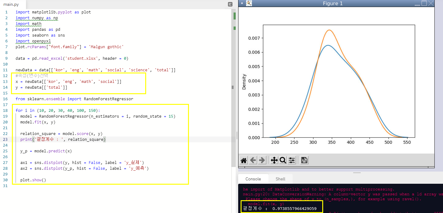
x에 국, 수, 사, 영을 넣어주고
n_estimators를 10, 20, 30, 40, 100, 150 으로 넣어가면서 각각의 결정계수를 확인해준다.
import matplotlib.pyplot as plot
import numpy as np
import math
import pandas as pd
import seaborn as sns
import openpyxl
plot.rcParams["font.family"] = 'Malgun gothic'

data = pd.read_excel('student.xlsx', header = 0)

newData = data[['kor', 'eng', 'math', 'social', 'science', 'total']]
#속성(변수)선택
x = newData[['kor', 'eng', 'math', 'social']]
y = newData[['total']]

from sklearn.ensemble import RandomForestRegressor

for i in (10, 20, 30, 40, 100, 150):
  model = RandomForestRegressor(n_estimators = i, random_state = 15)
  model.fit(x, y)

  relation_square = model.score(x, y)
  print('결정계수 : ', relation_square)

  y_p = model.predict(x)

  ax1 = sns.distplot(y, hist = False, label = 'y_실제')
  ax2 = sns.distplot(y_p, hist = False, label = 'y_예측')

  plot.show()
트리가 10, 20, 30, 40, 100, 150일때 각각
결정계수 : 0.9738557966429059
결정계수 : 0.9718858271579351
결정계수 : 0.9666089242741718
결정계수 : 0.966769981253321
결정계수 : 0.9659313535311665
결정계수 : 0.9648583441186911
이 나왔고 이 경우 오히려 트리가 10일때가 결정계수가 가장 높다.
4개의 성적으로 총점을 예측하는 것은 SVR 모델이 훨씬 결정계수가 높다.
SVR의 경우 거의 99.999%로 예측이 되었다.
예측 모델 중 갑은 SVR인듯하다.
'프로그래밍 > 머신러닝' 카테고리의 다른 글
| k-근접 모델(KNeighborsRegressor)_파이썬으로 머신러닝 배우기 (0) | 2021.04.29 |
|---|---|
| 그레이디언트 부스팅(GradientBoostingRegressor)_파이썬으로 머신러닝 배우기 (0) | 2021.04.26 |
| 서포트 백터 머신(model = SVR(kernel = 'rbf', C=1000, gamma = 1000)_파이썬으로 머신러닝 배우기 (0) | 2021.04.23 |
| 서포트 백터 머신(from sklearn.svm import SVR)_파이썬으로 머신러닝 배우기 (1) | 2021.04.21 |
| 집값과 경기종합지수의 상관관계_파이썬으로 머신러닝 배우기 (0) | 2021.04.19 |


